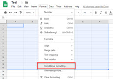
To do this, you just need to highlight the cell that you wanted to format conditionally, then on the menu bar click on format and click “Conditional Formatting.”

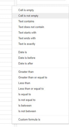
Then on the right pane click on add new rule. Apply to range shows the cells that have been highlighted and under “Format cells if…” you would see the conditions that are available. Just set the conditions based on your needs.

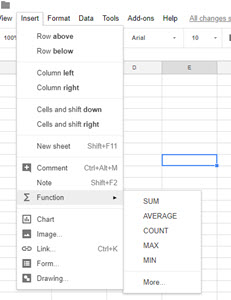
 To insert a formula first you need to select the cell where you want the answer to the formula to show up, then you click insert on the menu, then hover on “Function”, and you would see a list of formulas.

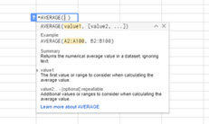
After selecting the formula, it would show you instructions on how to implement the formula.

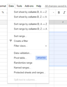
The third function is how to sort a list by alphabetical order. First, you need to make sure that you select all of the data, especially the rows. Then you click on data at the menu bar and select “sort range by column,” choose whether the column should be arranged from A-Z or vice versa. It will then change the order, and the rows would follow if you have highlighted it from before.

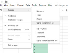
The last thing that I want to show you as an advance function of google sheets is how to freeze the panes. A lot of times, when you had a lot of data on the spreadsheet, you have to keep on scrolling, it is sometimes confusing especially when you got a label on the column, and you have to remember what is the name of that column is. All you have to do is click on “View” on the menu bar and hover on “Freeze,” you would get an option to freeze the rows or columns.